index
Introduction
These notes collect the core ideas from Lecture 1: what linear equations are, how to recognize and solve them, and how systems of such equations relate to geometry.
Linear equations
Definition (Linear Equation) A linear equation in variables x 1 , … , x n x_1,\dots,x_n x 1 , … , x n
a 1 x 1 + a 2 x 2 + ⋯ + a n x n = b , a_1x_1+a_2x_2+\cdots+a_nx_n=b, a 1 x 1 + a 2 x 2 + ⋯ + a n x n = b , where all a i a_i a i b b b
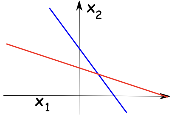
Figure1: None of those wave can be coefficient
Solutions
Definition (Solution) A solution is a list ( s 1 , … , s n ) (s_1,\dots,s_n) ( s 1 , … , s n ) ( x i = s i ) (x_i=s_i) ( x i = s i )
a 1 s 1 + a 2 s 2 + ⋯ + a n s n = b . a_1s_1+a_2s_2+\cdots+a_ns_n=b. a 1 s 1 + a 2 s 2 + ⋯ + a n s n = b .
Example
0.1 ⋅ 90 + 0.15 ⋅ 75 + 0.15 ⋅ 85 + 0.6 ⋅ 95 = 90
0.1\cdot 90+0.15\cdot 75+0.15\cdot 85+0.6\cdot 95=90 0.1 ⋅ 90 + 0.15 ⋅ 75 + 0.15 ⋅ 85 + 0.6 ⋅ 95 = 90 Hence 90 , 75 , 85 , 95 90,75,85,95 90 , 75 , 85 , 95 0.1 x 1 + 0.15 x 2 + 0.15 x 3 + 0.6 x 4 = 90 0.1x_1+0.15x_2+0.15x_3+0.6x_4=90 0.1 x 1 + 0.15 x 2 + 0.15 x 3 + 0.6 x 4 = 90
Lines (two variables)
Starting with slope–intercept form y = m x + b y=mx+b y = m x + b
y = m x + b ⟺ − m x + y = b y=mx+b \iff -mx+y=b y = m x + b ⟺ − m x + y = b which is a linear equation a 1 x 1 + a 2 x 2 = b a_1x_1+a_2x_2=b a 1 x 1 + a 2 x 2 = b x 1 = x x_1=x x 1 = x x 2 = y x_2=y x 2 = y a 1 = − m a_1=-m a 1 = − m a 2 = 1 a_2=1 a 2 = 1
Thus any equation a 1 x 1 + a 2 x 2 = b a_1x_1+a_2x_2=b a 1 x 1 + a 2 x 2 = b ( a 1 , a 2 ) ≠ ( 0 , 0 ) (a_1,a_2)\neq(0,0) ( a 1 , a 2 ) = ( 0 , 0 ) line in the plane, and a pair ( s 1 , s 2 ) (s_1,s_2) ( s 1 , s 2 )
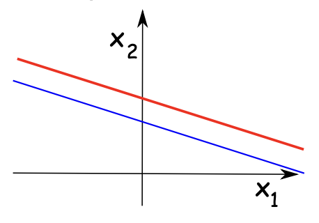
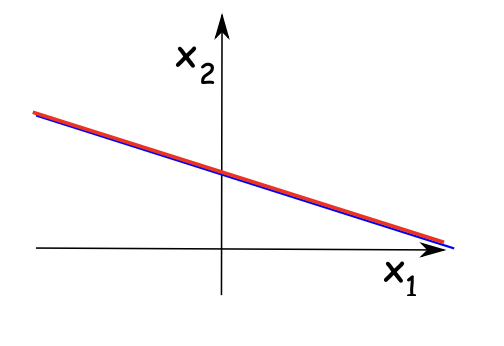
Figure2: Linear Equation and Lines
Linear Eq. System
Definition (Linear System) A system of m m m n n n
a 11 x 1 + a 12 x 2 + ⋯ + a 1 n x n = b 1 a 21 x 1 + a 22 x 2 + ⋯ + a 2 n x n = b 2 ⋮ a m 1 x 1 + a m 2 x 2 + ⋯ + a m n x n = b m \begin{aligned}
a_{11}x_1+a_{12}x_2+\cdots+a_{1n}x_n&=b_1 \\
a_{21}x_1+a_{22}x_2+\cdots+a_{2n}x_n&=b_2 \\
\vdots \\
a_{m1}x_1+a_{m2}x_2+\cdots+a_{mn}x_n&=b_m
\end{aligned} a 11 x 1 + a 12 x 2 + ⋯ + a 1 n x n a 21 x 1 + a 22 x 2 + ⋯ + a 2 n x n ⋮ a m 1 x 1 + a m 2 x 2 + ⋯ + a mn x n = b 1 = b 2 = b m A solution is a list s 1 , … , s n ∈ R n s_1,\dots,s_n\in\mathbb{R}^n s 1 , … , s n ∈ R n all equations simultaneously.
Geometric intuition
Each equation is a line; solving the system means finding the intersection of the lines.
Example
{ x 1 + 2 x 2 = 3 , 2 x 1 + x 2 = 3 ⟹ ( x 1 , x 2 ) = ( 1 , 1 ) .
\begin{cases}
x_1+2x_2=3,\\
2x_1+x_2=3
\end{cases}
\quad\Longrightarrow\quad (x_1,x_2)=(1,1).
{ x 1 + 2 x 2 = 3 , 2 x 1 + x 2 = 3 ⟹ ( x 1 , x 2 ) = ( 1 , 1 ) . Three outcomes are possible for a system of linear equations:
No solution (parallel, distinct lines) — inconsistent .
Exactly one solution (lines intersect at one point).
Infinitely many solutions (same line; solutions are parameterized ).
Matrices for a system
Extract the numbers into matrices.
A = [ a 11 a 12 ⋯ a 1 n a 21 a 22 ⋯ a 2 n ⋮ ⋮ ⋱ ⋮ a m 1 a m 2 ⋯ a m n ]
A=\begin{bmatrix}
a_{11}&a_{12}&\cdots&a_{1n}\\
a_{21}&a_{22}&\cdots&a_{2n}\\
\vdots&\vdots&\ddots&\vdots\\
a_{m1}&a_{m2}&\cdots&a_{mn}
\end{bmatrix} A = a 11 a 21 ⋮ a m 1 a 12 a 22 ⋮ a m 2 ⋯ ⋯ ⋱ ⋯ a 1 n a 2 n ⋮ a mn [ A ∣ b ] = [ a 11 a 12 ⋯ a 1 n b 1 a 21 a 22 ⋯ a 2 n b 2 ⋮ ⋮ ⋱ ⋮ ⋮ a m 1 a m 2 ⋯ a m n b m ] [A|\mathbf{b}]=
\left[
\begin{array}{cccc|c}
a_{11}&a_{12}&\cdots&a_{1n}&b_1\\
a_{21}&a_{22}&\cdots&a_{2n}&b_2\\
\vdots &\vdots &\ddots&\vdots &\vdots\\
a_{m1}&a_{m2}&\cdots&a_{mn}&b_m
\end{array}
\right] [ A ∣ b ] = a 11 a 21 ⋮ a m 1 a 12 a 22 ⋮ a m 2 ⋯ ⋯ ⋱ ⋯ a 1 n a 2 n ⋮ a mn b 1 b 2 ⋮ b m These capture all the information needed to solve the system.
Elementary Row Operations (EROS)
The following row operations do not change the solution set of a system:
Row interchange : swap two rows.Row scaling : multiply a row by a nonzero constant c c c Row replacement : replace a row by itself plus c c c
Using EROS to simplify [ A ∣ b ] [A|\mathbf{b}] [ A ∣ b ] Gaussian elimination - Keep repeating this process until it’s in reduced row-echelon form (RREF) to get solutions.
Gaussian elimination
Solve
{ x + 2 y = 3 2 x + y = 3 ⟺ [ 1 2 3 2 1 3 ]
\begin{cases}
x+2y=3\\
2x+y=3
\end{cases}
\quad\Longleftrightarrow\quad
\left[\begin{array}{cc|c}
1&2&3\\
2&1&3
\end{array}\right] { x + 2 y = 3 2 x + y = 3 ⟺ [ 1 2 2 1 3 3 ] Apply EROS:
R 2 ← R 2 − 2 R 1 : [ 1 2 3 0 − 3 − 3 ] R 2 ← − 1 3 R 2 : [ 1 2 3 0 1 1 ] R 1 ← R 1 − 2 R 2 : [ 1 0 1 0 1 1 ]
\begin{aligned}
R_2 \leftarrow R_2-2R_1&:
\left[\begin{array}{cc|c}
1&2&3\\
0&-3&-3
\end{array}\right]
\\
R_2 \leftarrow -\tfrac13 R_2&:
\left[\begin{array}{cc|c}
1&2&3\\
0&1&1
\end{array}\right]
\\
R_1 \leftarrow R_1-2R_2&:
\left[\begin{array}{cc|c}
1&0&1\\
0&1&1
\end{array}\right]
\end{aligned}
R 2 ← R 2 − 2 R 1 R 2 ← − 3 1 R 2 R 1 ← R 1 − 2 R 2 : [ 1 0 2 − 3 3 − 3 ] : [ 1 0 2 1 3 1 ] : [ 1 0 0 1 1 1 ] Thus x = 1 , y = 1 x=1,\ y=1 x = 1 , y = 1
Summary
A linear equation a 1 x 1 + ⋯ + a n x n = b a_1x_1+\cdots+a_nx_n=b a 1 x 1 + ⋯ + a n x n = b line (n = 2 n=2 n = 2 plane (n = 3 n=3 n = 3 hyperplane (n > 3 n>3 n > 3
Solutions to a system are the intersection of these hyperplanes.
A system has no solution , one solution , or infinitely many solutions .
Use matrices and EROS (Gaussian elimination) to simplify to echelon / RREF and get solutions.
Adapted from the source lecture PDF.
 Figure1: None of those wave can be coefficient
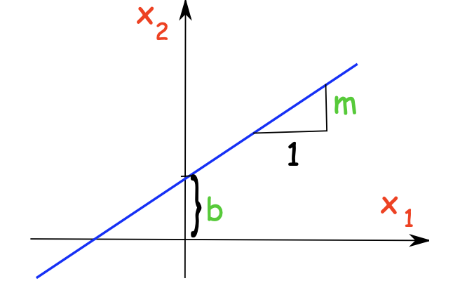 Figure2: Linear Equation and Lines